
Data Analysis Plugins#
Note
This is the config-specific version of documentation and is deprecated. See the general documentation for the most up-to-date information.
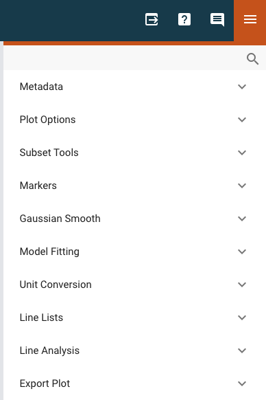
The Specviz data analysis plugins are meant to aid quick-look analysis of 1D spectroscopic data. All plugins are accessed via the plugin icon in the upper right corner of the Specviz application. These plugins are built upon specutils to do the actual analysis work
Any spectra generated by plugins (e.g., Gaussian Smooth) will be automatically displayed in the spectral viewer. These spectra, and any other that is available, can be found in the data selection dropdown menu (see Selecting Data Set for more detail) where you can also toggle their visibility. This functionality is also available through the Python API.
Metadata Viewer#
See also
- Metadata Viewer
Imviz documentation on using the metadata viewer.
Plot Options#
See also
- Spectral Plot Options
Documentation on further details regarding the plot setting controls.
Subset Tools#
See also
- Subset Tools
Imviz documentation describing the concept of subsets in Jdaviz. Subsets in Specviz are strictly spectral subsets and do not support rotation or recentering.
Markers#
See also
- Markers
Imviz documentation describing the markers plugin.
Gaussian Smooth#
Gaussian Smooth convolves a Gaussian function (kernel) with a Spectrum data object to smooth the data. The convolution requires a Gaussian standard deviation value (in pixels) which can be entered into the Standard deviation field in the plugin.
A new Spectrum object is generated and is added to the spectrum viewer. The object can be selected and shown in the viewer via the Data icon in the viewer toolbar.
Model Fitting#
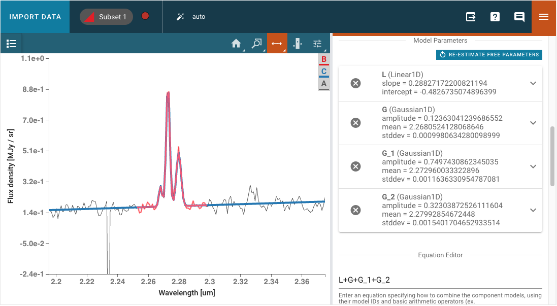
Astropy models can be fit to a spectrum via the Model Fitting plugin. Model components are selected via the Model Component pulldown menu. The Add Component button adds a Model Components block.
Model Parameters are automatically initialized with a guess. These starting values can be edited by the user. They may also be fixed by selecting the checkbox, so that they are not fit or changed by the model fitting.
A mathematical expression must be entered into the Equation Editor to specify the mathematical combination of models. This is also necessary even if there is only one model component. The model components are specified by their labels and the equation defaults to the sum of all created components, but can be modified to exclude some of components without needing to delete them entirely or to change to subtraction, for example. The user can also select a different fitter to use for the model and adjust the corresponding parameters that appear in the Fitter Parameters accordion menu. The default fitter used is astropy.modeling.fitting.TRFLSQFitter. The fitter can be changed to any of the available Astropy fitters, which can be found here https://docs.astropy.org/en/latest/modeling/reference_api.html#id6.
After fitting, the expandable menu for each component model will update to show the fitted value of each parameter rather than the initial value, and will additionally show the standard deviation uncertainty of the fitted parameter value if the parameter was not set to be fixed to the initial value and if the spectrum uncertainty was loaded.
Note
When a 1D Spline Models. model is selected, the plugin uses
astropy.modeling.spline.SplineSmoothingFitter. to compute the fit.
The initial value of the smoothing factor is automatically set to:
(len(data) * (standard_deviation(data))**2).
Refer to the section of the Scipy spline modeling documentation explaining
the s parameter for advice on setting the smoothing factor/condition manually:
https://docs.scipy.org/doc/scipy/reference/generated/scipy.interpolate.UnivariateSpline.html#scipy.interpolate.UnivariateSpline
From the API#
The model fitting plugin can be run from the API:
# Open model fitting plugin
plugin_mf = specviz.plugins['Model Fitting']
plugin_mf.open_in_tray()
# Input the appropriate dataset and subset
plugin_mf.dataset = 'my spectrum'
plugin_mf.spectral_subset = 'Subset 1'
# Input the model components
plugin_mf.create_model_component(model_component='Linear1D',
                                 model_component_label='L')
plugin_mf.create_model_component(model_component='Gaussian1D',
                                 model_component_label='G')
# Set the initial guess of some model parameters
plugin_mf.set_model_component('G', 'stddev', 0.002)
plugin_mf.set_model_component('G', 'mean', 2.2729)
# Model equation gets populated automatically, but can be overwritten
plugin_mf.equation = 'L+G'
# Set fitter
plugin_mf.fitter.selected = 'TRFLSQFitter'
# Calculate fit
plugin_mf.calculate_fit()
Customizing Fitter Parameters#
The fitter parameters (such as maximum iterations, filtering non-finite values, etc.)
can be accessed and modified programmatically using the
get_fitter_parameter()
and set_fitter_parameter()
methods. The available parameters depend on the selected fitter.
Common parameters include:
maxiter: Maximum number of iterations (available for most fitters)filter_non_finite: Whether to filter non-finite values like NaNs (available for most fitters)calc_uncertainties: Whether to calculate parameter uncertainties (available for most fitters)
# Get the current value of a fitter parameter
max_iterations = plugin_mf.get_fitter_parameter('maxiter')
print(f"Current max iterations: {max_iterations}")

# Set a new value for a fitter parameter
plugin_mf.set_fitter_parameter('maxiter', 200)
plugin_mf.set_fitter_parameter('filter_non_finite', False)

# Verify the change
new_max_iterations = plugin_mf.get_fitter_parameter('maxiter')
print(f"New max iterations: {new_max_iterations}")
Note that different fitters support different parameters. For example, LinearLSQFitter
does not support the maxiter parameter. If you attempt to get a parameter that doesn’t
exist for the selected fitter, the method will return None.
Exporting Fit Results#
Parameter values for each fitting run are stored in the plugin table.
To export the table into the notebook, call
export_table()
(see Accessing Plugin APIs).
See also
- Export Models
Documentation on exporting model fitting results.
Unit Conversion#
The spectral flux density and spectral axis units can be converted using the Unit Conversion plugin.
Select the frequency, wavelength, or energy unit in the Spectral Unit pulldown (e.g., Angstrom, Hertz, erg).
Select the flux density unit in the Flux Unit pulldown (e.g., Jansky, W/Hz/m2, ph/Angstrom cm2 s).
Note that this affects the default units in all viewers and plugins, where applicable, but does not affect the underlying data.
From the API#
The Unit Conversion plugin can be called from the API:
unitconv_pl = specviz.plugins['Unit Conversion']
unitconv_pl.spectral_unit = 'Angstrom'
Line Lists#
Line wavelengths can be plotted in the spectrum viewer using the Line Lists plugin.
Line lists (e.g. Common Stellar, SDSS, CO) can be selected from Preset Line Lists via the Available Line Lists pulldown. They are loaded and displayed by pressing Load List. Each loaded list is shown under Loaded Lines and can be be removed manually.
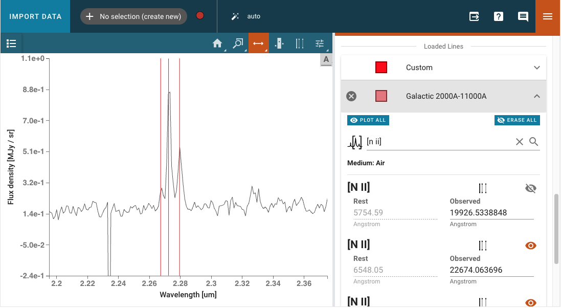
Loaded Lines includes a Custom line list which is automatically created, but populated with no lines. Lines may be added to the Custom line list by entering Line Name, Rest Value, and Unit for the spectral axis and pressing Add Line. Selected lines may be hidden by deselecting the associated check box.
The color of each line list may be adjusted with the color and saturation sliders. Entire line lists may be hidden in the display via Show All and Hide All, located at the bottom of each list. Similarly, all of the line lists may be shown or hidden via Plot All and Erase All, located at the bottom of the plugin.
Importing Custom Line Lists#
Jdaviz comes with curated line lists built by the scientific community. If you cannot find the lines you need, you can add your own by constructing an astropy table. For example:
from astropy.table import QTable
from astropy import units as u

my_line_list = QTable()
my_line_list['linename'] = ['Hbeta','Halpha']
my_line_list['rest'] = [4851.3, 6563]*u.AA

viz.load_line_list(my_line_list)
# Show all imported line lists
viz.spectral_lines
Redshift Slider#
Warning
Using the redshift slider with many active spectral lines causes performance issues. If the shifting of spectral lines lag behind the slider, try plotting fewer lines. You can deselect lines using, e.g., the “Erase All” button in the line lists UI.
The Line Lists plugin also contains a redshift slider which shifts all of the plotted lines according to the provided redshift/RV. The slider applies a delta-redshift, snaps back to the center when releasing, and has limits that default based on the x-limits of the spectrum viewer. This provides a convenient method to fine-tune the position of the redshifted lines to the observed lines in the spectrum.
From the API#
The range and step size of the slider can be set from a notebook cell using the
set_redshift_slider_bounds()
method in Specviz by specifying the range or step keywords, respectively.
Setting either keyword to 'auto' means its value will be calculated
automatically based on the x-limits of the spectrum plot.
The redshift itself can be set from the notebook using the set_redshift method.
Any set redshift values are applied to spectra output using the
get_spectra() helper method.
Note that using the lower-level app data retrieval (e.g., specviz.get_data())
will return the data as originally loaded, with the redshift unchanged.
Line Analysis#
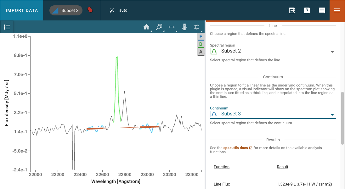
The Line Analysis plugin returns specutils analysis for a single spectral line. The line is selected via the region tool in the spectrum viewer to select a spectral subset. Note that you can have multiple subsets in Specviz, but the plugin will only show statistics for the selected subset.
A linear continuum is fitted and subtracted (divided for the case of equivalenth width) before computing the line statistics. By default, the continuum is fitted to a region surrounding the select line. The width of this region can be adjusted, with a visual indicator shown in the spectrum plot while the plugin is open. The thick line shows the linear fit which is then interpolated into the line region as shown by a thin line. Alternatively, a custom secondary region can be created and selected as the region to fit the linear continuum.
The properties returned include the line centroid, gaussian sigma width, gaussian FWHM, total flux, and equivalent width. Uncertainties on the derived properties are also returned. For more information on the algorithms used, refer to the specutils documentation.
The line flux results are automatically converted to Watts/meter2, when appropriate.
From the API#
The Line Analysis plugin can be run from the API:
# Open line analysis plugin
plugin_la = specviz.plugins['Line Analysis']
plugin_la.open_in_tray()
# Input the appropriate spectrum and region
plugin_la.dataset = 'my spectrum'
plugin_la.spectral_subset = 'Subset 2'
# Input the values for the continuum
plugin_la.continuum = 'Subset 3'
# Return line analysis results
plugin_la.get_results()
Redshift from Centroid#
Following the table of statistics, the centroid can be used to set the redshift by assigning
the centroid value to a line added in the Line List Plugin. Select the
corresponding line from the dropdown, or by locking the selection to the identified line and
using the ![]() (line selector) tool in the spectrum viewer.
(line selector) tool in the spectrum viewer.
Export#
This plugin allows exporting the contents of a viewer or a plot within a plugin to various image formats. Additionally, spatial and spectral (Astropy) regions can be exported to files. Spatial regions may be exported as either FITS or REG files while Spectral regions may be exported as ECSV files. Note that multiple spectral regions can be saved to the same file so long as they are subregions of a single subset rather than independent subsets.